Changing Initial Concentrations the easy way

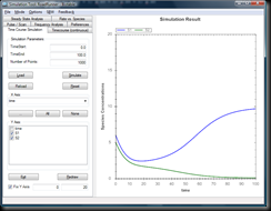
It’s been some time since I updated the SBW Simulation Tool, just to jog the Memory the SBW Simulation Tool, is the application, that will interact with all SBW enabled Simulators and makes it a snap to perform simulation experiments (be it time course simulations, steady state computations, pulse or scan experiments or even Frequency Analysis). Especially neat, if you ask me, is the Options\Slider feature, which basically attaches a handle to all parameters / boundary conditions of a model and allows you to quickly modify the current value and see what effect it has on the simulation you were performing.

Changing parameters and boundary conditions was great, but what about initial concentrations of all the floating species. Of course that is an operation that should have been there in the first place, and so *drum roll* here finally a version that makes it a snap to modify those values as well. So lets try it, lets take a simple bi-stable model like this one:

p = defn Bistable

var S1, S2;

$X0 => S1; k1*(1+x)/(1+k2*pow(S2,2));
$X0 => S2; k3/(1+k4*pow(S1,2));

S1 => $X0; k0*S1;
S2 => $X0; k0*S2;

end;
// initialize Parameters
p.k1 = 1; p.k2 = 1; p.k3 = 1; p.k4 = 1; p.k0 = 0.1;

// and initial conditions
p.S1 = 5; p.S2 = 5;

You’d paste the model above simply into JarnacLite and then click SBW\Simulation Tool: RoadRunner to get it into the simulator. And then select Options\Sliders … and now if you vary the initial conditions of S2 you see how the behavior changes … amazing, isn’t it?

Here the result for S1 = 4

and S1 = 6

Neat … just as an aside … remember to check the “Fix Y Axis” Checkbox! otherwise the experience is limited, as the graph will scroll the whole time to adapt to the values.